Using Everest

There are two ways of interacting with the everest catalog: via the command line and through the Python interface. For quick visualization, check out the everest and estats command line tools. For customized access to de-trended light curves in Python, keep reading!

A Simple Example

Once you’ve installed everest, you can easily import it in Python:

import everest

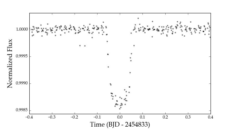
Say we’re interested in EPIC 201367065, a K2 transiting exoplanet host star. Let’s instantiate the Everest class for this target:

star = everest.Everest(201367065)

You will see the following printed to the screen:

INFO  [everest.user.DownloadFile()]: Downloading the file...
INFO  [everest.user.load_fits()]: Loading FITS file for 201367065.

Everest automatically downloaded the light curve and created an object containing all of the de-trending information. For more information on the various methods and attributes of star, check out the everest.Detrender documentation (from which Everest inherits a bunch of parameters) and the Everest docstring.

To bring up the DVS (data validation summary) for the target, execute

star.dvs()

You can also plot it interactively:

star.plot()

The raw light curve is shown at the top and the de-trended light curve at the bottom. The 6 hr CDPP (a photometric precision metric) is shown at the top of each plot in red. Since this light curve was de-trended with a break point, which divides it into two separate segments, the CDPP is shown for each one. At the top, below the title, we indicate the CDPP for the entire light curve (raw → de-trended). Outliers are indicated in red, and arrows indicate points that are beyond the limits of the plot (zoom out to see them). You can read more about these plots here.

Finally, if you want to manipulate the light curve yourself, the timeseries is stored in star.time and star.flux (PLD-de-trended flux) or star.fcor (de-trended flux with CBV correction). The indices of all outliers are stored in star.mask.

Masking Transits

If you’re using everest for exoplanet/eclipsing binary science, you will likely want to apply a mask to any transits in the light curve to prevent them from getting washed out by the least-squares fitting step. The de-trended light curves provided in the catalog automatically mask large outliers, but it is still strongly recommended that all transits be masked during the de-trending step to minimize de-trending bias. This can be done easily and quickly as follows:

star.mask_planet(t0, per, dur = 0.2)
star.compute()

where t0 is the time of first transit, per is the period, and dur is the full transit duration (all in days).

Alternatively, you can specify directly which indices in the light curve should be masked by setting the star.transitmask attribute:

star.transit_mask = np.array([0, 1, 2, ...], dtype = int)
star.compute()

Note that this does not overwrite outlier masks, which are stored in the star.outmask, star.badmask, and star.nanmask arrays.

Note

You must run the compute method for the model to be re-trained on the out-of-transit data. Running compute typically takes a few seconds. For short cadence light curves, it may take a minute or two.

Transit Search & Optimization

Masking the transits is one way to prevent overfitting and improve the de-trending power, but it can be somewhat inelegant. Oftentimes, one may not know when (or if!) transits occur in a light curve, so masking them ahead of time is not possible. Fortunately, the fact that everest is a linear model makes it easy to simultaneously optimize the transit and the instrumental components, ensuring that the PLD model won’t try to fit out transits (and that the transit model won’t latch on to systematics). There are two ways to go about this simultaneous fit in everest.

The first is to explicitly include a transit model in the PLD design matrix—which means we treat the transit model like an additional regressor and solve for its weight (which is just the transit depth). This will give you the maximum likelihood (ML) solution for the transit depth, if the other transit properties (period, time of first transit, impact parameter, etc.) are known.

model = everest.TransitModel(name, **kwargs)
star.transit_model = model
star.compute()

See everest.transit.TransitModel for the available keyword arguments. After running compute, the ML transit depth is stored in star.transit_depth.

The method above may be of limited use, particularly when the transit times and shape are not precisely known. Moreover, although it is possible to obtain the uncertainty on the ML solution for the depth, that uncertainty isn’t really that meaningful, since it doesn’t take into account any uncertainty in the PLD model; instead, it is the uncertainty on the depth when the likelihood of the PLD model is maximized. Usually, a much better approach is to compute the transit depth that maximizes the marginal likelihood; this depth is what you get when you marginalize (integrate over) the uncertainty on all of the parameters of the model. Luckily, for a linear model it is easy (and super fast) to compute the marginal likelihood. In everest, all you need to do is

m = model(star.time)
lnlike, depth , vardepth = star.lnlike(m, full_output=True)

where model is the same transit model as above. The variable depth is the depth that maximizes the marginal likelihood under the given transit model, and vardepth is its variance (the square of the standard deviation on the estimate of the depth).

Under this framework, we can go a step further: say we don’t know the other transit model parameters, such as the period, the times of transit, or if there’s any transit present to begin with. Since we have a fast way of computing the marginal likelihood (lnlike above), we can use it to obtain posterior distributions for the parameters of interest. Since the transit model is not linear in any of these other parameters, we need to use approximate methods, such as MCMC (Markov Chain Monte Carlo), to obtain the posteriors. 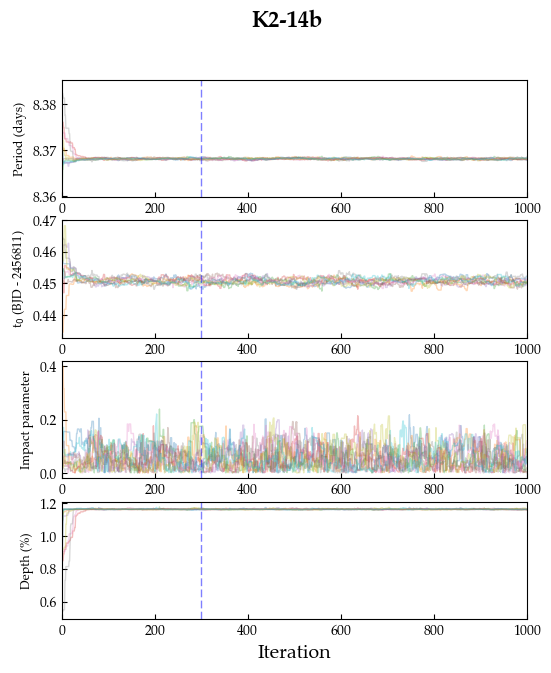Check out the mcmc.py script for an example in which the properties of K2-14b are estimated based on evaluating the marginal likelihood. The basic idea is to define our likelihood as a function of the transit parameters (in this case, the period, the time of first transit, and the impact parameter):

def lnlike(x, star):
    """Return the log likelihood given parameter vector `x`."""
    per, t0, b = x
    model = TransitModel('b', per=per, t0=t0, b=b)(star.time)
    ll = star.lnlike(model)
    return ll

where star = everest.Everest(201635569) and use the emcee package to run an MCMC chain to obtain the posterior distributions of these parameters. Here’s what the chains look like, for 10 walkers and 1000 iterations (~5 minutes on my laptop):

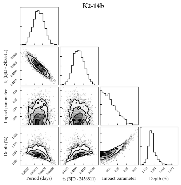
And here’s the posterior distributions after discarding the first 300 steps as burn-in:

In general, this is going to be somewhat slower than computing the maximum likelihood estimate – such as what you do when you fit for the transit parameters given the “de-trended” light curve. But the beauty here is that we are never “de-trending” – we are performing inference on the original dataset given information about the nature of the noise (the covariance matrix). This will lead to more robust posterior distributions, less overfitting, and more realistic uncertainties on the transit parameters. If possible, the “de-trend-then-search” method should be avoided and this should be done instead!

CBV Corrections

The everest pipeline automatically corrects de-trended light curves with a single co-trending basis vector (CBV) calculated from all the de-trended light curves observed during that season/campaign. The CBV-corrected flux is stored in star.fcor and is the quantity that is plotted by default when the user calls star.plot() (the uncorrected, de-trended flux is star.flux).

Sometimes, it is desirable to correct the light curve with a different number of CBVs. For K2, everest calculates 5 CBVs for each campaign, so any number from 0-5 is possible. To correct the light curve with 2 CBVs, run

star.cbv_num = 2
star.compute()

Plotting the light curve will now show the flux corrected with two CBVs.

Note

The everest catalog uses only 1 CBV to prevent fitting out real astrophysical variability. Care must be taken when using more CBVs to ensure this is not the case.

Here is an example of EPIC 201367065 corrected with 0, 1, 2, 3, and 4 CBVs. Note that the fourth CBV appears to introduce extra variability; at that point, the correction is likely overfitting.

Number of CBVs	De-trended light curve
0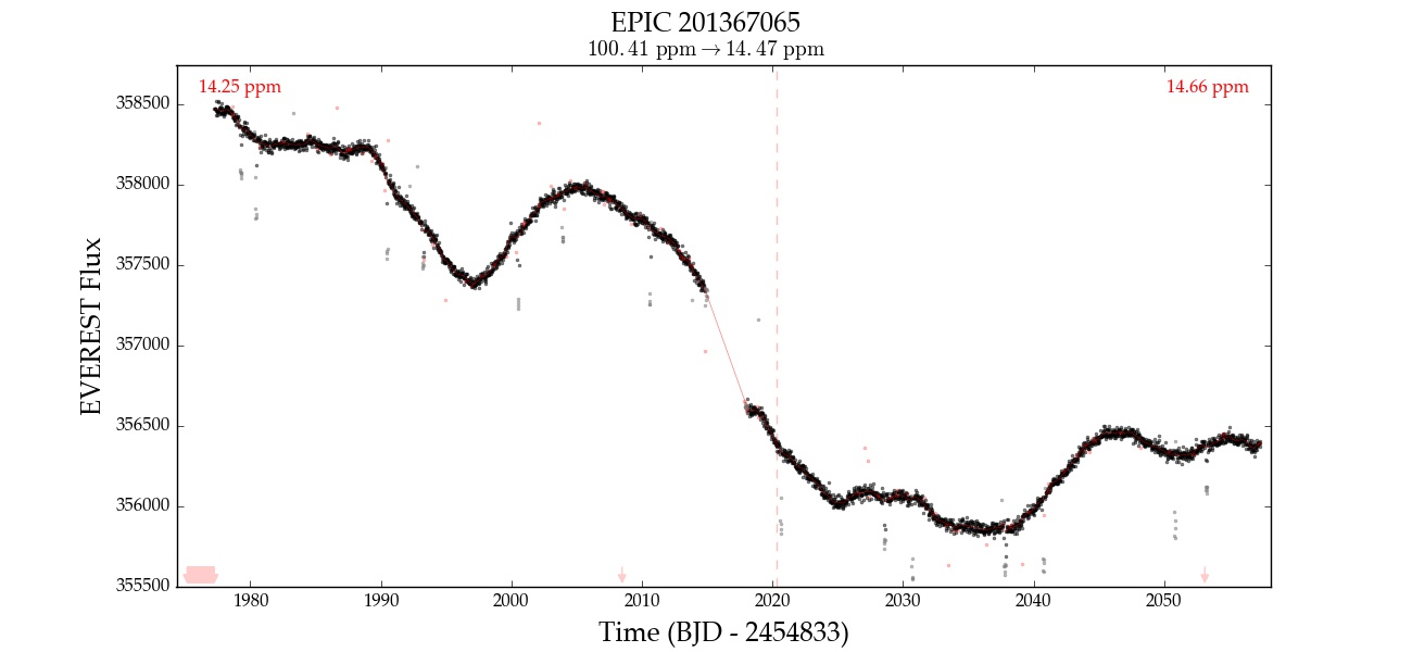
1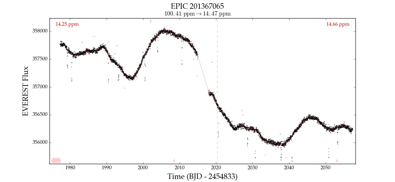
2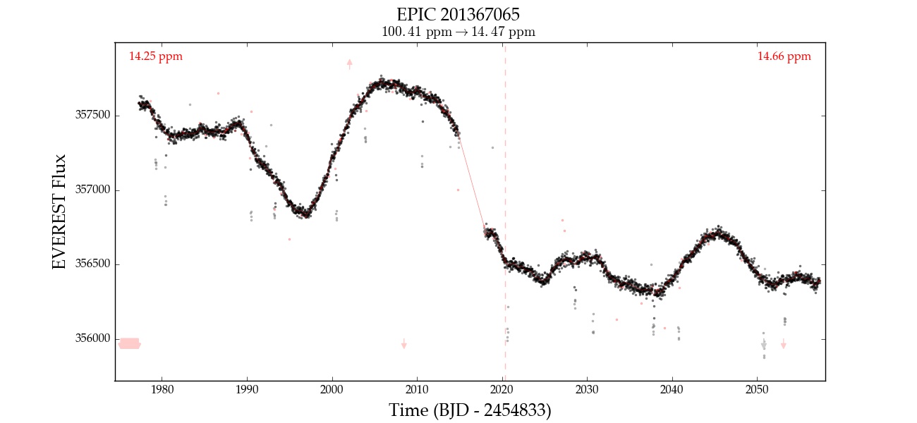
3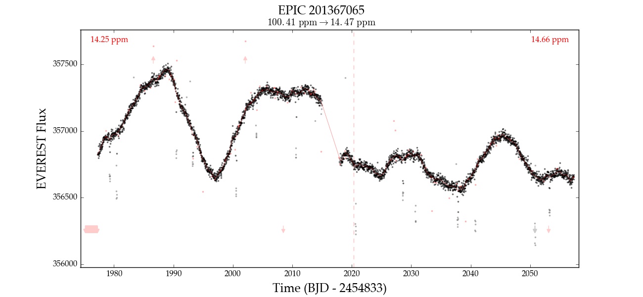
4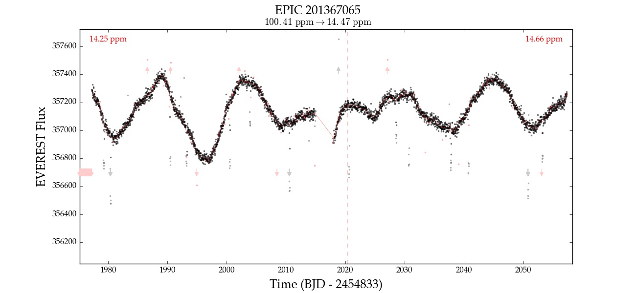

Note

The CBVs are stored as column vectors in the star.XCBV design matrix.

Tuning the Model

The cross-validation step seeks to find the optimal value of the regularization parameter lambda for each PLD order. These are stored in the star.lam array, which has shape (nsegments, pld_order). Changing these numbers will change the PLD weights and thus the de-trending power, but it will likely lead to underfitting/overfitting. Nevertheless, in cases where the optimization fails, tweaking of these numbers could be useful. Here’s the star.lam array for EPIC 201367065:

[[3.16e05, 3.16e11, 1.0e11],
 [1.00e09, 1.00e09, 1.e09]]

We can compute the second order PLD model by zeroing out the third order elements:

star.lam = [[3.16e05, 3.16e11, 0.],
            [1.00e09, 1.00e09, 0.]]
star.compute()

Pipeline Comparison

It’s easy to plot the light curve de-trended with different pipelines:

star.plot_pipeline('everest1')
star.plot_pipeline('k2sff')
star.plot_pipeline('k2sc')

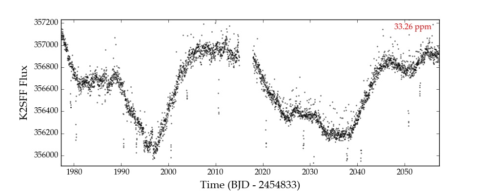
Here’s EPIC 201367065 de-trended with K2SFF:

Folded Transits

If there are transits/eclipses in a light curve, everest can use the GP prediction to whiten the timeseries and fold it on the period of the planet. If the time of first transit and period of an exoplanet/EB are known, plotting the folded transit/eclipse is easy. Just remember to mask the transit and re-compute the model beforehand:

star.mask_planet(1980.42, 10.054)
star.compute()
star.plot_folded(1980.42, 10.054)

Custom Detrending

As of version 2.0.9, users can de-trend their own raw K2 FITS files using the everest.standalone.DetrendFITS() function, which is a wrapper for the everest.detrender.rPLD detrender.

Overfitting Metrics

As we discussed above, everest() is known to overfit transits when they are not properly masked. Users can now compute an estimate of the degree of overfitting in any light curve by typing

everest 201601162 -o

into a terminal. This will compute and plot two overfitting metrics: the unmasked overfitting metric and the masked overfitting metric. Both correspond to the fractional decrease in a transit depth due to overfitting and are computed by running transit injection/recovery tests at every cadence in a light curve. For EPIC 201601162, computing these metrics took about 2 minutes on my laptop. Here is what a snippet of the diagnostic plot looks like:

The top panel shows the unmasked overfitting metric: the degree of overfitting when transits are not masked. This is evaluated at every cadence. The distribution of values is shown as the histogram at the right, indicating a median overfitting of 0.07 (7%), with a typical spread (median absolute deviation, or MAD) of 0.036 (3.6%). The bottom panel shows the masked overfitting metric: the degree of overfitting when transits are masked (see above). This is much smaller and is zero on average, indicating that everest does not overfit when transits are excluded from the regression.

The actual PDF has several more rows, corresponding to the overfitting metrics for different injected transit depths. In general, overfitting gets worse the lower the signal-to-noise ratio of the light curve.